Audio-Reactive Visuals using Generative AI: Our First Exploration with VAEs
- Sophia Bouchama
- Jun 18, 2023
- 13 min read
Updated: Jun 21, 2023
ASHA FM is delving into the realm of generative AI, and it’s time to share a demo of the first iteration of one of our innovations.
How our AI Journey Began
Our AI journey began at Le Wagon London, a Data Science bootcamp where myself, Jack, Maadhav and Matea all met. We were a group of individuals with varied backgrounds, but shared a common interest and love for art, music and technology.
Our paths crossed during a group project challenge where we were tasked to develop an AI-based project in just 10 days. Maadhav had a vision to create an online radio, delivering an audio streaming platform generating the visuals using AI. His idea came about during the Covid pandemic, when he could no longer run his sound system events and the scene was put on hold. The proposal of his idea led us as a group to be motivated into bringing this into reality. After many hours of research, we found it difficult to find published audio-visual platforms that cultivated music and AI in the format we envisioned. Motivated by this challenge, we decided to create something of our own, that intersected the spheres of art and AI - a generative AI model that syncs to the beat of music.


ASHA FM Data Science Team: Working and Coding
The days leading up to the demo were intense but rewarding. We dedicated countless hours to perfecting our project. On demo day, we presented our project, a testament to our collective effort, dedication and support of the wonderful community and teaching staff at Le Wagon. The result was a AI-powered visual experience, generated by a Variational AutoEncoder deep learning model (more on that later), that complemented the dynamic beats of any audio input. As we dug deeper into the world of deep learning models and generative art, we became more excited about the potential our project held, which is what led us to drive ASHA FM forward and launch as an online creative platform after receiving positive feedback and interest.

ASHA FM Data Science Team: Project Demo Day at Le Wagon
From left to right: Jack Sibley, Matea Miljevic, Sophia Bouchama and Maadhav Kothari
Brief Project Overview
Gather image data, provided to us by graphic designer and visual artist Sean Zelle.
Utilise a deep learning model (Variational AutoEncoder) to generate a series of novel images based on the original dataset that will serve as individual frames for the video.
Create smooth transitions between the AI-generated images to form a dynamic video.
Extract audio features from a chosen audio track.
Use these audio features to manipulate the transitions between the images, providing an audio-reactive effect to the video.
Assemble all these AI-curated and manipulated images to form the final product: an audio-reactive video.
The Technical Side
Choosing the Right Model
VAES
After deliberation on various neural network models, we decided on a VAE (Variational AutoEncoder). A VAE is a type of generative model that is used for creating new, original data that resembles the input data it's trained on. It's capable of transforming and generating complex data such as images, making it a good fit for our purpose.
VAEs have an additional advantage in terms of providing a more explicit probabilistic framework for modeling the data distribution than other neural network models such as GAN (Generative Adversarial Networks) or a regular AutoEncoder. They are designed to learn a probability distribution (usually Gaussian) over the input data and then generate new samples by sampling from this learned distribution.
VAEs are built using an encoder-decoder architecture with a well defined latent space and a reconstruction loss, allowing for more explicit control over the generation process and easier interpretation of the latent variables. Having a defined latent space was crucial to assisting our goal in making the transition between images audio reactive - this is where the data manipulation would take place.
Regular AutoEncoders don't explicitly model the distribution of the data at all. They learn to copy their inputs to their outputs, with a bottleneck layer in between that forces them to learn a compressed representation of the data. However, without the probabilistic modeling aspect, the representations learned by regular AutoEncoders might not be as meaningful as those learned by VAEs.
GANS
While GANs can also generate high quality images, they work in a different way. They consist of two neural networks: a generator, which creates new images, and a discriminator, which tries to distinguish between real and generated images. The generator does not have an explicit encoding step that maps inputs to a latent space. Instead, it learns to transform random noise vectors into images that can ‘trick’ the discriminator.
Because of this different approach, the latent space in GANs is typically less interpretable than in VAEs. The absence of a clear mapping from inputs to points in the latent space means that it can be more difficult to understand what each dimension of the latent space represents. This makes the latent space of GANs less intuitive to work with. Considering our time and resource constraints, VAE seemed like our best option.
Latent space
Each point in this latent space corresponds to a latent vector (representing a potential image) consisting of a specified number of dimensions. These dimensions can be thought of as 'features' that the VAE model uses to effectively encapsulate the complexity of an image. Higher dimensions can allow for a more detailed representation of the data, but also runs the risk of the model overfitting.
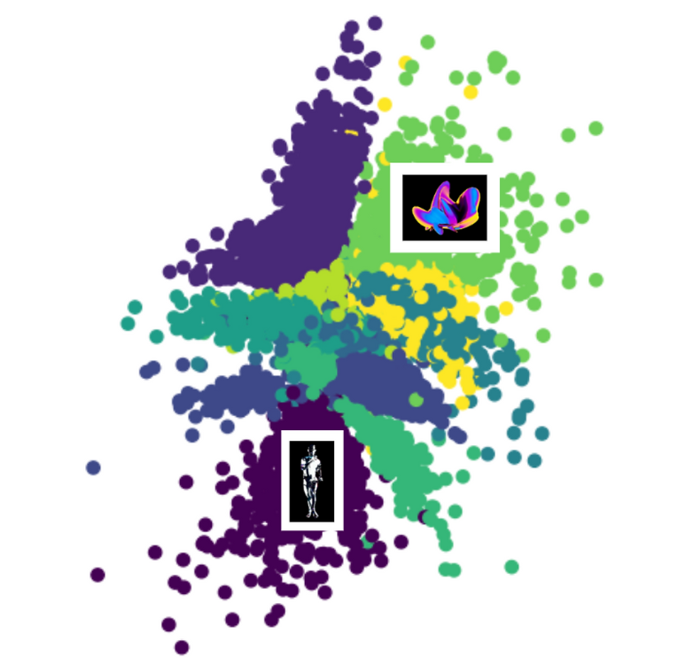
In our case, the choice of 200 latent dimensions was a balance to prevent the model from overfitting or underfitting. It allowed us to capture sufficient detail to generate visually accurate images without overly complicating the model. This is one of the many parameters that we had to experiment with in order to achieve a desired result.
When we interpolate between two points (or latent vectors) in this space, we're creating a series of images that smoothly transition from one image to another. So, in relation to our work with the VAE model, we are encoding our images into this latent space and then smoothly transitioning or interpolating between these points to create a video that corresponds with the changes in our music.
VAE Architecture
The VAE model consists of two parts: an Encoder (with a sampling layer) and a Decoder.
Please see our GitHub project for reference.

Encoder
The encoder's function is to take an input (in our case, an image) and convert it into a compact, latent representation. This representation captures the important features of the input data.
Our encoder is composed of several layers of Convolutional Neural Networks (CNNs), which successively downsample the image until it is a flat vector (i.e a tensor). This flat vector is then used to generate two things - a vector of means (z_mean) and a vector of variances (z_log_var). A custom Sampling layer generates a new vector 'z' by adding a random noise scaled by the variance to the mean.
Probabilistic Sampling in VAE
The heart of a VAE is the 'Sampling' layer, where we introduce randomness into the model. Given the 'z_mean' and 'z_log_var' vectors from the encoder, we generate a 'z' vector by adding a random element. This element, epsilon, is a random tensor sampled from a normal distribution.
The purpose of this random sampling is to allow the model to generate diverse outputs even when it's fed with the same input. This is a crucial property for generative models, enabling them to produce different but plausible data instances.
The Variational AutoEncoder is a generative model that employs deep learning techniques to not only learn efficient representations of input data but also generate new instances from the learned space. Unlike traditional AutoEncoders, which learn to compress data and reconstruct it without considering the data distribution, VAEs introduce a probabilistic spin that ensures the learned latent space is smooth and meaningful.
Decoder
The decoder takes this latent representation 'z' and reconstructs the original data from it. To accomplish this, it upsamples 'z' using a series of Convolutional Transpose layers until it regenerates an image of the original shape. This reconstructed image is the final output of our VAE. This reconstruction process is essentially the inverse of what the encoder does.
During training, the VAE learns to optimise these two processes. The encoder learns to generate a meaningful latent representation that captures the necessary information, while the decoder learns to recreate the original input from this representation.
Our Model Architecture
Since we coded our own VAE instead of using a pre-trained model, let's delve a bit deeper into the technical details of our encoder-decoder architecture. Experimentation of the architecture and parameters is necessary to achieve our desired outcome.
Breakdown of the Encoder
The first layer of our CNN takes an input image of shape 448x448x3. It applies 32 filters of size 3x3, using the 'ReLU' activation function and 'same' padding (which ensures the output has the same length as the original input). The layer is followed by a 2x2 max-pooling layer which reduces the dimensions of the image.
The next set of layers repeat this process with increasing numbers of filters (64, 128, 256). Each convolutional layer is followed by a max-pooling layer which further reduces the image dimensions.
The output from these layers is then flattened to a one-dimensional tensor.
The flattened tensor is then passed to two separate dense layers, creating a mean vector (z_mean) and a variance vector (z_log_var).
Finally, a custom Sampling layer generates a vector 'z' by adding random noise, scaled by the variance, to the mean.
The idea behind this architecture is to gradually reduce the spatial dimensions of the input while increasing the depth, capturing more complex features at each layer.
Breakdown of the Decoder
The decoder starts with a Dense layer which takes the latent vector as input and produces a tensor of shape (7, 7, 128).
This tensor is then passed through a series of Convolutional Transpose layers. These layers do the opposite of what Convolutional layers do - they increase the spatial dimensions and decrease the depth of the input.
The Convolutional Transpose layers use the ReLU activation function and 'same' padding, similar to the encoder.
The number of filters in each Convolutional Transpose layer gradually decreases, mirroring the structure of the encoder.
The final layer uses a sigmoid activation function to produce a tensor that can be interpreted as an image, matching the dimensions of the original input image.
The decoder learns to reverse the process of the encoder, using the latent representation 'z' to reconstruct the original input as closely as possible.
Training the VAE and Loss Functions
Training the VAE involves defining a loss function composed of two components: the reconstruction loss and the KL divergence.
The total loss is a combination of these two losses, and the weights of the VAE are updated to minimise this total loss. This kind of architecture allows our model to generate new, unique data, similar to the original input data.
Reconstruction Loss
This measures how well the decoder is able to reconstruct the original input data from the latent space. ensures that the input and the output of the VAE (the original image and the reconstructed image) are as close as possible. In other words, it checks the fidelity of the output against the original data.
KL Divergence
Named after Kullback-Leibler, this loss measures how much the learned latent variables deviate from the standard normal distribution. Essentially, it's a form of regularisation that ensures the latent space has good properties that allow efficient generation of new instances. The KL divergence is a measure of how closely the learned latent distribution aligns with a standard normal distribution.
The total loss of the VAE model, which we aim to minimize during training, is the sum of these two components. It's through this training process and the interplay between the encoder and decoder components that VAEs learn to generate new data instances that are similar to the ones in their training set.


Examples of Our VAE Model's Progress Across Different Iterations
How do we Create Audio-Reactive Visuals?
The VAE architecture allows for the creation of visuals based on input images. When paired with audio analysis and beat detection, we can alter the encoded 'z' vector based on different audio parameters such as onset times or beat strengths. This results in visual representations that are directly reactive to the audio input, thereby achieving the sought after audio-visual experience.
Spleeter is an open-source project by Deezer. It is a Python library that allows you to take an audio file and separate it into its component tracks. For example, if you have a song file, you could separate the vocals from the backing track, or you could separate the drums, bass, vocals, and other instruments into separate audio files. This gives us control over what aspects of the track we want to base the transitions on.
In order to create audio-reactive visuals, we make use of Python's Librosa library which allows us to analyse audio signals and extract useful information such as beat timings. Here's how we achieve this:
Extracting Audio Parameters: We begin by loading our audio file with a sample rate of 22050 Hz. We then calculate the duration of the audio in seconds and the total number of frames.
Onset Info Extraction: Next, we load the audio once again with a different sample rate that ensures the total number of frames matches with the video frames. We then determine the onset strength of each beat. The 'onset' of a sound is the start of a musical note or sound, which is typically characterised by a distinct increase in the sound wave's amplitude. We also determine the onset times and frames and combine this information into an array.
Beat Time Extraction: We then use one of the library functions to detect beat times in the audio. A beat is the basic time unit of a piece of music, and these are usually the elements of the music that you tap your foot along to.
Creating Onset Features: Once we have our onset information and beat times, we proceed to create onset features. These features are used to create a visual reaction every time a beat is detected in the audio. If the current time corresponds to a beat, we set the corresponding value in the feature array to the onset strength of that beat. This value then decays linearly or exponentially over time until the next beat occurs. The speed of decay can be adjusted using the linear decay time and exponential decay rate parameters that we have defined.
Applying Decay: The idea behind decay is to gradually decrease the effect of a beat as time passes, creating a sense of rhythm in the visuals. Linear decay achieves this by subtracting a fixed value at each step, while exponential decay multiplies the current value by a fixed factor, leading to a faster decrease initially that slows down over time. By adjusting the parameters for the decay rates, this enables us to fine-tune the visuals.

These steps allow us to create an array of features that react to the beats in our audio. These features are then used to modify the generated visuals, creating a dynamic, audio-reactive visual experience. The visuals will intensify with the strength of the beat and then gradually decay, keeping in sync with the rhythm of the music.
Linear and exponential decay are methods used to gradually decrease the intensity of a value over time. In the context of audio-reactive visuals, these methods are used to create a sense of rhythm and dynamics in the visuals, making them respond to the beats in the music in a way that feels natural and engaging. Here's a more detailed look at both methods:

Linear Decay: In linear decay, a fixed amount is subtracted from the value at each step. This results in a steady decrease over time. If you were to graph it, it would form a straight line. In our context, linear decay is used to gradually lessen the visual impact of a beat as time progresses until the next beat occurs. The visual intensity associated with a beat will decrease at a constant rate, regardless of how strong or weak the beat was.
Exponential Decay: In exponential decay, the value is multiplied by a fixed factor at each step. This results in a rapid decrease at first that slows down over time. The graph of an exponential decay is a curve that starts off steep and gradually flattens out. In terms of the visuals, exponential decay creates a stronger immediate reaction to a beat that then tapers off more slowly. This can make the visuals feel more responsive and dynamic, especially for music with a lot of strong, rapid beats.
Transforming Encoded Images into Interpolated Vectors
Once we have our encoded images, we need to create transitions between each image. This is where interpolation comes into play. We wrote a function to perform either linear or exponential interpolation between neighboring images, guided by the audio's onset information.
We take two vectors in the latent space (i.e two images to move between) then create a step vector that incrementally moves us from the start to the end. How we move in the latent space from one image to another is determined by the features of the audio extracted. For each frame in the gap between two images, we add a scaled version of the step vector to our starting vector, with the scale factor derived from the audio's onset information. We calculate these vectors for both linear and exponential transitions.
Combining Interpolated Images with Audio into a Video
Now, we just need to combine this series of interpolated images with the audio to create our final music video.
We create a function reads in the audio file, set its duration, and then creates a sequence of frames from the interpolated images.
The frames are chained together to form a continuous video clip, and then the audio is overlaid.
Finally, the combined video and audio is saved to the specified location. The end result is a music video where the images transition smoothly in sync with the audio. This approach offers a novel way of visualising the intricate relationship between audio and visuals.
Short Demo: Our Initial Prototype of Audio-Reactive AI Visuals
What’s Next?
Overall, this VAE model forms the core of our audio-reactive visual art generation, but we still have a lot of hurdles to overcome.
As we move forward in our exploration of VAE models and consideration of other models that we would like to try such as StyleGAN, there are some key areas where we'll be focusing our attention to further improve the capabilities and efficiency.
The main issue being computational limitations as deep learning models are computationally intensive. The vast amount of data that needs to be processed, and the complexity of the tasks involved, mean that training these models, rendering longer videos, and increasing the resolution of the images all require significant computing resources.
One of the primary constraints we face is the limitation of GPU capacity. Graphics Processing Units (GPUs) have been instrumental in advancing machine learning because of their ability to process multiple computations concurrently. This is particularly vital when it comes to deep learning models like StyleGAN, which involve large amounts of matrix and vector operations. However, as we strive to train larger models and produce higher quality outputs, we are increasingly pushing the boundaries of what current GPUs can handle.
As we continue to advance in this field, AI image synthesis is promising, but the road ahead is not without its challenges. The key lies in our ability to continue innovating and pushing the boundaries of what's possible, even as we grapple with the computational limits of our current technology to further enrich our platform's creative space.
We always welcome collaboration, new ideas, and proposals. Please feel free to get in touch with us info@asha.fm.
You can watch our live demo and presentation here (skip to 1:59:40), and all our code can be viewed on GitHub.
Follow us at ASHA FM for more updates and projects.
Sophia Bouchama is a data scientist whose experience spans across various aspects of the tech space, ranging from digital design to software engineering and consultancy. She can be reached on LinkedIn and Instagram.


